A Closer Look At The Advanced CODAS Moving Average Algorithm
Versatile moving average in Advanced CODAS algorithm filters waveform noise, extracts mean, and eliminates baseline drift.
The moving average is a simple mathematical technique used primarily to eliminate aberrations and reveal the real trend in a collection of data points. You might be familiar with it from averaging noisy data in a freshman physics experiment, or from tracking the value of an investment. You might not know that the moving average is also a prototype of the finite impulse response filter, the most common type of filter used in computer-based instrumentation. In cases where a given waveform is cluttered with noise, where a mean needs to be extracted from a periodic signal, or where a slowly drifting baseline needs to be eliminated from a higher frequency signal, a moving average filter may be applied to achieve the desired result. The moving average algorithm of Advanced CODAS offers this kind of waveform filtering performance. Advanced CODAS is an analysis software package that operates on existing waveform data files created by first generation WinDaq or second generation WinDaq data acquisition packages. In addition to the moving average algorithm, Advanced CODAS also includes a report generator utility and software routines for waveform integration, differentiation, peak and valley capturing, rectification, and arithmetic operations.
Moving Average Filter Theory
DATAQ Instruments' moving average algorithm allows a great deal of flexibility in waveform filtering applications. It can be used as a low-pass filter to attenuate the noise inherent in many types of waveforms, or as a high-pass filter to eliminate a drifting baseline from a higher frequency signal. The procedure used by the algorithm to determine the amount of filtering involves the use of a smoothing factor. This smoothing factor, controlled by you through the software, can be increased or decreased to specify the number of actual waveform data points or samples that the moving average will span. Any periodic waveform can be thought of as a long string or collection of data points. The algorithm accomplishes a moving average by taking two or more of these data points from the acquired waveform, adding them, dividing their sum by the total number of data points added, replacing the first data point of the waveform with the average just computed, and repeating the steps with the second, third, and so on data points until the end of the data is reached. The result is a second or generated waveform consisting of the averaged data and having the same number of points as the original waveform.

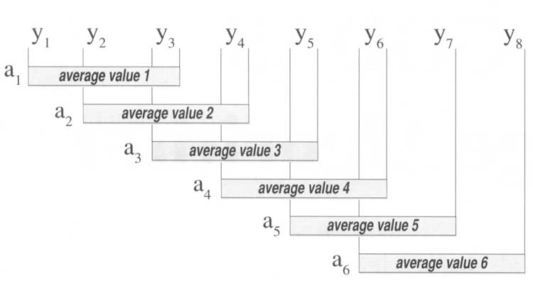
Figure 1 — Any periodic waveform can be thought of as a long string or collection of data points. In the above illustration, consecutive waveform data points are represented by "y" to illustrate how the moving average is calculated. In this case, a smoothing factor of three was applied, which means three consecutive data points from the original waveform are added, their sum divided by three, and then this quotient is plotted as the first data point of a generated waveform. The process repeats with the second, third, and so on data points of the original waveform until the end of the data is reached. A special "feathering" technique averages the beginning and end data points of the original wave-form to ensure that the generated waveform contains the same number of data points as the original.
Figure 1 illustrates how the moving average algorithm is applied to waveform data points (which are represented by y). The illustration features a smoothing factor of 3, which means that the average value (represented by a) will be calculated over 3 consecutive waveform data values. Note the overlap that exists in the moving average calculations. It is this overlapping technique, along with a special beginning- and end-point treatment that generates the same number of data points in the averaged waveform as existed in the original.
The way the algorithm calculates a moving average deserves a closer look and can be illustrated with an example. Say we have been on a diet for two weeks and we want to compute our average weight over the last 7 days. We would sum our weight on day 7 with our weight on days 8, 9, 10, 11, 12, and 13; and then multiply by 1/7. To formalize the process, this can be expressed as:
a(7) = 1/7(y(7) + y(8) + y(9) + ... + y(13))
This equation can be further generalized. The moving average of a waveform can be calculated by:
![]()
Where:
a = averaged value
n = data point position
s = smoothing factor
y = actual data point value

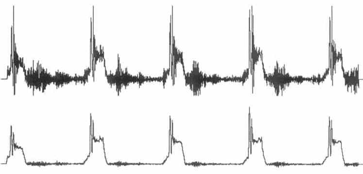
Figure 2* — The load cell output waveform shown original and unfiltered in the top channel and as an 11-point moving averaged waveform in the bottom channel. The noise appearing on the original waveform was due to the intense vibrations created by the press during the packaging operation.
The key to this algorithm's flexibility is its wide range of selectable smoothing factors (from 2 - 1,000). The smoothing factor determines how many actual data points or samples will be averaged. Specifying any positive smoothing factor simulates a low-pass filter while specifying a negative smoothing factor simulates a high-pass filter. Given the absolute value of the smoothing factor, higher values apply greater smoothing constraints on the resulting waveform and conversely, lower values apply less smoothing. With the application of the proper smoothing factor, the algorithm can also be used to extract the mean value of a given periodic waveform. A higher positive smoothing factor is typically applied for generating mean waveform values.
Applying the Moving Average Algorithm
A salient feature of the moving average algorithm is that it can be applied many times to the same waveform if necessary to get the desired filtering result. Waveform filtering is a very subjective exercise. What may be a properly filtered waveform to one user may be unacceptably noisy to another. Only you can judge whether the number of averaged points selected was too high, too low, or just right. The flexibility of the algorithm allows you to adjust the smoothing factor and make another pass through the algorithm when satisfactory results are not achieved with the initial attempt.
The application and capabilities of the moving average algorithm can be illustrated best by the following examples.

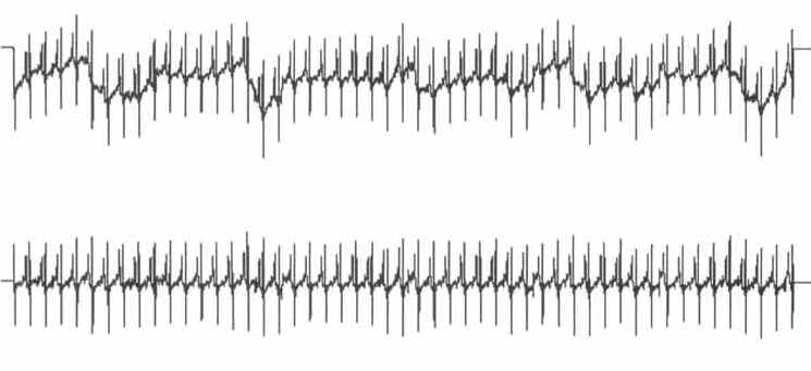
Figure 3* — The ECG waveform shown original and unfiltered in the top channel and as a 97-point moving averaged waveform in the bottom channel. Note the absence of baseline drift in the bottom channel. Both waveforms are shown in a compressed condition for presentation purposes.
A Noise Reduction Application
In cases where a given waveform is cluttered with noise, the moving average filter may be applied to suppress the noise and yield a clearer picture of the waveform. For example, an Advanced CODAS customer was using a press and a load cell in a packaging operation. Their product was to be compressed to a predetermined level (monitored by the load cell) to reduce the size of the package required to contain the product. For quality control reasons, they decided to monitor the press operation with instrumentation. An unexpected problem appeared when they began viewing the real-time load cell output. Since the press machine vibrated considerably while in operation, the load cell's output waveform was difficult to discern because it contained a large amount of noise due to the vibration as shown in the top channel of Figure 2. This noise was eliminated by generating an 11-point moving averaged channel as shown in the bottom channel of Figure 2. The result was a much clearer picture of the load cell's output.
An Application in Eliminating Baseline Drift
In cases where a slowly drifting baseline needs to be removed from a higher frequency signal, the moving average filter may be applied to eliminate the drifting baseline. For example, an ECG waveform typically exhibits some degree of baseline wander as can be seen in the top channel of Figure 3. This baseline drift can be eliminated without changing or disturbing the characteristics of the waveform as shown in the bottom channel of Figure 3. This is accomplished by applying an appropriate negative-value smoothing factor during the moving average calculation. The appropriate smoothing factor is determined by dividing one waveform period (in seconds) by the channel's sample interval. The channel's sample interval is simply the reciprocal of the channel's sample rate and is conveniently displayed on the moving average utility menu. The waveform period is easily determined from the display screen by positioning the cursor at a convenient point on the waveform, setting a time marker, and then moving the cursor one complete cycle away from the displayed time marker. The time difference between cursor and time marker is one waveform period and is displayed at the bottom of the screen in seconds. In our ECG example, the waveform possessed a channel sample interval of .004 seconds (obtained from the moving average utility menu) and one waveform period was measured to span .388 seconds. Dividing the waveform period by the channel's sample interval gave us a smoothing factor of 97. Since it is the baseline drift that we are interested in eliminating, we applied a negative smoothing factor (-97) to the moving average algorithm. This in effect subtracted the moving averaged result from the original waveform signal, which eliminated the baseline drift without disturbing waveform information.
Other Waveform Moving Average Issues
Whatever the application, the universal reason for applying a moving average filter is to "smooth out" the high and low aberrations and reveal a more representative intermediate waveform value. When doing this, the software should not compromise other features of the original waveform in the process of generating a moving averaged waveform. For example, the software should automatically adjust the calibration information associated with the original data file, so that the moving averaged waveform is in the appropriate engineering units when generated.
*All readings in the figures were taken using WinDaq Data Acquisition software


 View Cart
 sales@dataq.com
 330-668-1444